High-Fidelity 3D Scene Reconstruction Integrating Diffusion Models with Memory-Efficient Neural Radiance Fields

1. Overview

DiffusionNeRF-3D introduces a novel approach to 3D scene reconstruction by combining diffusion models with Neural Radiance Fields (NeRF). The project implements a two-stage pipeline that first uses a diffusion model to refine depth maps from RGBD images, which are then used by a memory-efficient NeRF model for high-quality 3D scene reconstruction. This integration addresses key limitations in traditional NeRF approaches, particularly for scenes with complex geometry or limited view coverage. The system was developed and evaluated using the NYU Depth V2 dataset, which provides RGB-D images of diverse indoor scenes.

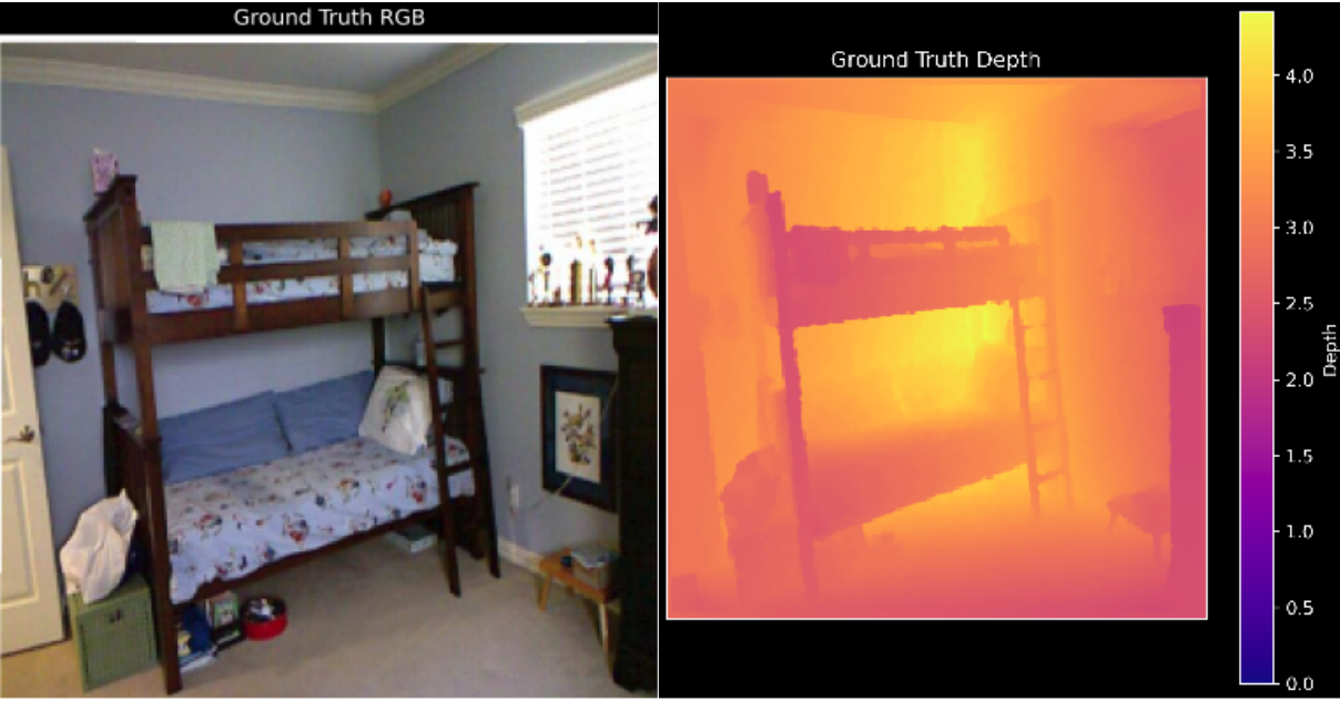
Example from NYU Depth V2 dataset showing RGB image (left) and corresponding depth map (right) used for training and evaluation

2. Technical Approach

The first stage of the pipeline uses a specialized diffusion model to enhance the quality of depth maps:

UNet Architecture: Implemented with multi-scale feature processing, attention mechanisms at bottleneck, and feature enhancement blocks
Training Strategy: Cosine noise scheduling with advanced edge-aware loss functions
Key Components:
- Group normalization for stable training
- Residual connections for improved gradient flow
- Feature enhancement blocks for detail preservation

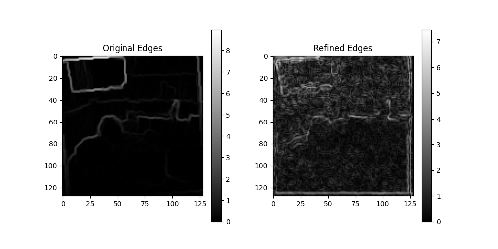
Edge-aware processing comparing original edges (left) with refined edges (right), demonstrating the preservation of structural details

The diffusion model was designed to progressively denoise corrupted depth maps while maintaining critical edge information and structural details. This is particularly important for preserving geometric boundaries in complex indoor scenes.

def _compute_edge_loss(self, pred, target):
    """Compute edge-aware loss between prediction and target with robust grid handling."""
    def _get_edges(x):
        """Get edges using Sobel filters with robust grid size handling."""
        # Implementation details omitted for brevity
        sobel_x = torch.tensor([[-1, 0, 1], 
                            [-2, 0, 2], 
                            [-1, 0, 1]], device=x.device).float()
        sobel_y = torch.tensor([[-1, -2, -1],
                            [0, 0, 0],
                            [1, 2, 1]], device=x.device).float()
        
        # Apply filters and compute edge magnitudes
        edges_x = F.conv2d(x, sobel_x)
        edges_y = F.conv2d(x, sobel_y)
        edges = torch.sqrt(edges_x.pow(2) + edges_y.pow(2) + 1e-6)
        
        return edges
    
    # Compute losses on extracted edges
    pred_edges = _get_edges(pred)
    target_edges = _get_edges(target)
    edge_loss = F.l1_loss(pred_edges, target_edges)
    return edge_loss

2.2 Memory-Efficient NeRF Implementation

The second stage leverages a custom Neural Radiance Field (NeRF) implementation with several optimizations:

Efficient Encoding: Implemented hash encoding for faster training and better detail preservation
Performance Optimizations:
- Occupancy grid acceleration to skip empty space
- Gradient checkpointing to reduce memory usage
- Mixed precision training for improved throughput
Advanced Training: Integrated depth supervision from the diffusion model with custom loss functions

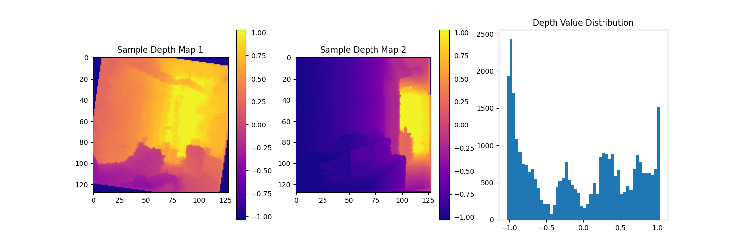
Depth value distribution analysis showing the distribution of depth values across the dataset, helping to calibrate model parameters

The NeRF implementation features a sophisticated volumetric rendering approach:

def render_rays(self, model, rays_o, rays_d, near, far, depth_prior=None):
    """Volumetric rendering for a batch of rays."""
    with torch.set_grad_enabled(self.training):
        device = rays_o.device
        batch_size, n_rays = rays_o.shape[:2]
        
        chunk_size = 1024
        outputs = []
        
        for i in range(0, n_rays, chunk_size):
            chunk_rays_o = rays_o[:, i:i+chunk_size]
            chunk_rays_d = rays_d[:, i:i+chunk_size]
            chunk_out = self._render_rays_chunk(
                model, chunk_rays_o, chunk_rays_d, near, far, depth_prior
            )
            outputs.append(chunk_out)
        combined = {}
        for k in outputs[0].keys():
            combined[k] = torch.cat([out[k] for out in outputs], dim=1)
        
        return combined

This implementation includes advanced sampling techniques to efficiently distribute samples along each ray:

def sample_pdf(bins, weights, n_samples, det=False):
    """Sample points from probability distribution given by weights.
    
    This is for sampling points according to their importance during ray marching.
    PDF here means "Probability Density Function" which helps focus samples 
    where they're most needed.
    """
    weights = weights.float()
    bins = bins.float()
    weights = weights + 1e-5
    pdf = weights / torch.sum(weights, dim=-1, keepdim=True)
    
    cdf = torch.cumsum(pdf, dim=-1)  # [..., n_bins]
    cdf = torch.cat([torch.zeros_like(cdf[..., :1]), cdf], dim=-1)  # [..., n_bins+1]

    if det:
        u = torch.linspace(0., 1., n_samples, device=weights.device)
        u = u.expand(list(cdf.shape[:-1]) + [n_samples])
    else:
        u = torch.rand(list(cdf.shape[:-1]) + [n_samples], device=weights.device)

    u = u.contiguous()
    cdf = cdf.unsqueeze(-2).expand(*cdf.shape[:-1], n_samples, cdf.shape[-1])
    inds = torch.searchsorted(cdf[..., -1], u)
    below = torch.clamp(inds-1, min=0)
    above = torch.clamp(inds, max=cdf.shape[-1]-1)
    inds_g = torch.stack([below, above], -1)
    
    bins_expanded = bins.unsqueeze(-2).expand(*bins.shape[:-1], n_samples, bins.shape[-1])
    
    bins_g = torch.gather(bins_expanded, -1, inds_g)
    cdf_g = torch.gather(cdf, -1, inds_g)

    denom = cdf_g[..., 1] - cdf_g[..., 0]
    denom = torch.where(denom < 1e-5, torch.ones_like(denom), denom)
    t = (u - cdf_g[..., 0]) / denom
    samples = bins_g[..., 0] + t * (bins_g[..., 1] - bins_g[..., 0])
    
    return samples

3. Training Pipeline

The project includes a comprehensive training pipeline with several advanced techniques:

3.1 Diffusion Model Training

Scheduler: Implemented OneCycleLR with warmup for stable convergence
Loss Function: Combined MSE, edge-aware loss, and perceptual loss
Optimization: Early stopping with patience for optimal model selection
Augmentation: Designed multi-view consistency loss for better generalization

3.2 NeRF Training

Custom Loss Functions: Depth-aware losses with edge preservation terms
Gradient Management: Implemented gradient clipping and dynamic batch sizing
Memory Optimization: Integrated various techniques to reduce memory footprint:
- Ray chunking for processing large scenes
- Efficient data loading pipelines
- Gradient checkpointing to reduce memory during backpropagation

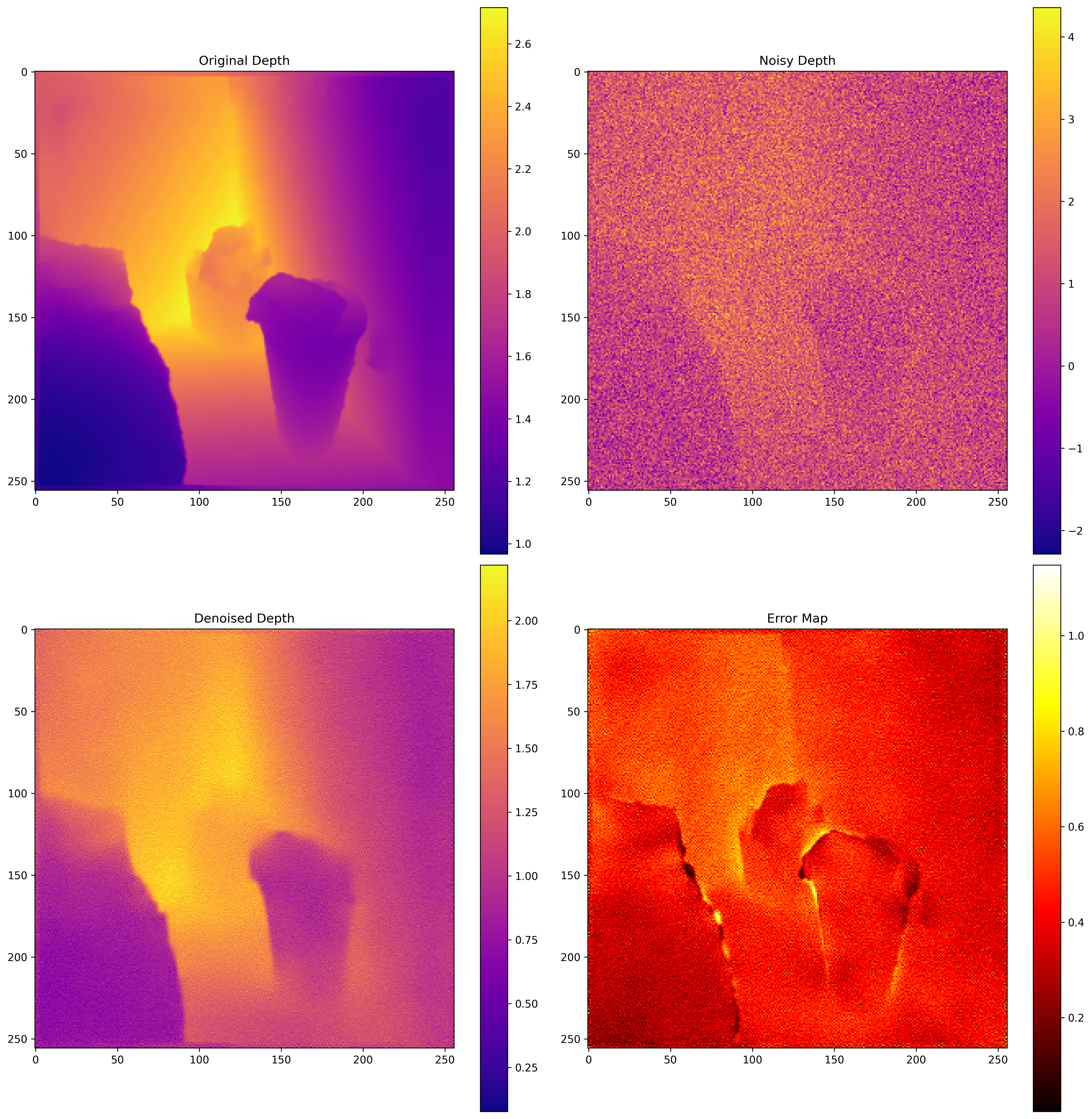
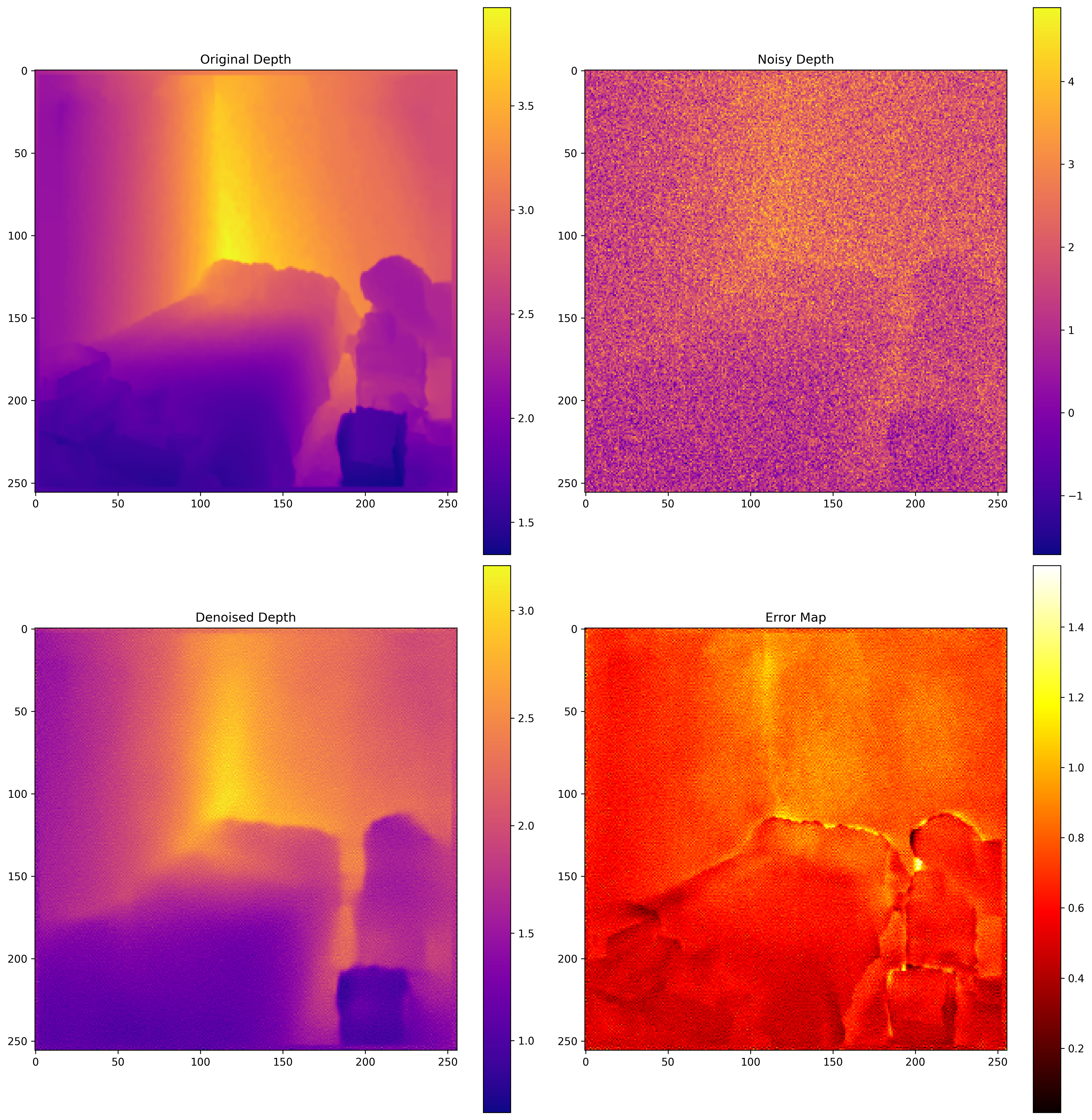
Additional examples of depth map refinement showing the model's ability to handle different scene types

4. Results and Performance

While this project is ongoing, initial results show promising performance:

Depth Refinement Metrics:
- MSE: 0.8901
- PSNR: 0.7254
Memory Efficiency: Successfully processes high-resolution inputs with limited GPU memory
Edge Preservation: Significantly improved edge preservation compared to baseline methods

The current implementation demonstrates the system’s ability to effectively:

Denoise and refine depth maps from consumer-grade depth cameras
Preserve critical structural information during the denoising process
Build consistent 3D reconstructions from the refined depth maps
Operate with reasonable memory requirements despite the complexity of the models

5. Future Directions

The project has several planned enhancements:

InstantNGP Techniques: Integrating additional techniques from InstantNGP for faster rendering
Sparse Voxel Grid Acceleration: Adding sparse voxel grid for further speed improvements
Interactive Viewer: Developing an interactive 3D viewer for real-time exploration
Multi-View Consistency: Enhancing the consistency between multiple viewpoints

6. Project Repository

DiffusionNeRF-3D